Slide 1

Slide notes: Job Costing BI is a part of Business Intelligence in IES, and provides additional capabilities to the Ledger BI, mostly for Project Costing and related Business Management.

Slide 2

Slide notes:

Slide 3

Slide notes: Views Sets are re-usable, and we may either start a new View Set, or select from available View Sets that we have created before. In this case, we will choose Manufacture to start our exercise with.

Slide 4

Slide notes: With the perspective of Production Manager, in a Company that Manufactures Juice, among other products, we will now evaluate the performance of our Juice Production runs for the month of August.

Slide 5

Slide notes:

Slide 6

Slide notes:

Slide 7

Slide notes: In a View Set, we always have selected period Settings for Current Year and Prior Year, and we can change these settings on demand to get any Period View that we want.

Slide 8

Slide notes:

Slide 9

Slide notes:

Slide 10

Slide notes: For a Job View, we can use 1 or more Flag Ranges to select the Jobs to include in the View. We may use lookups or intuitive searches to select these Flags, and to re-state the settings, we can easily use the initialize function and then start with fresh Flag setting selection.

Slide 11

Slide notes:

Slide 12

Slide notes:

Slide 13

Slide notes:

Slide 14

Slide notes:

Slide 15

Slide notes:

Slide 16

Slide notes:

Slide 17

Slide notes:

Slide 18

Slide notes:

Slide 19

Slide notes:

Slide 20

Slide notes:

Slide 21

Slide notes:

Slide 22

Slide notes:

Slide 23

Slide notes:

Slide 24

Slide notes:

Slide 25

Slide notes:

Slide 26

Slide notes:

Slide 27

Slide notes: Before opening a Job View, we indicate the View Perspective that we want. In fact, we can even define our own types of measurements also, which are then available in addition to the standard Cost Type measurements that are always present. Whatever we need to measure in Job Costing BI probably can be measured.

Slide 28

Slide notes:

Slide 29

Slide notes:

Slide 30

Slide notes:

Slide 31

Slide notes:

Slide 32

Slide notes:

Slide 33

Slide notes: With view number 301, we can select 2 Performance Measures on the right to be compared. So, to evaluate our Expenditure versus Budget on the Production Runs, we may select accordingly.

Slide 34

Slide notes:

Slide 35

Slide notes:

Slide 36

Slide notes:

Slide 37

Slide notes:

Slide 38

Slide notes:

Slide 39

Slide notes:

Slide 40

Slide notes:

Slide 41

Slide notes: In this view we can easily see on the Chart how the Production Runs have fared against the Budget, and the actual figures are listed below. For more detail, we can drill deeper into any of the listed Jobs.

Slide 42

Slide notes:

Slide 43

Slide notes: Next, we want to use an Asset Management View Set, so we will switch Views Sets.

Slide 44

Slide notes:

Slide 45

Slide notes:

Slide 46

Slide notes:

Slide 47

Slide notes:

Slide 48

Slide notes: Before we look at any of the Performance Measurements for these Asset Jobs, we will use a Cost Type View to reveal the Capital invested in these Assets.

Slide 49

Slide notes:

Slide 50

Slide notes:

Slide 51

Slide notes:

Slide 52

Slide notes:

Slide 53

Slide notes:

Slide 54

Slide notes:

Slide 55

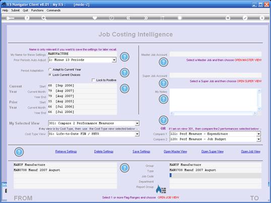
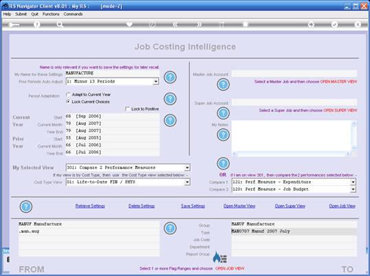
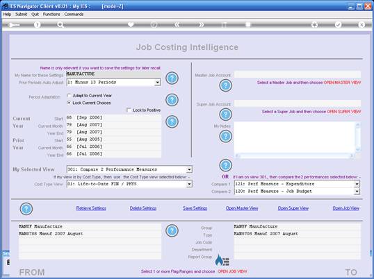
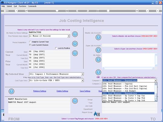
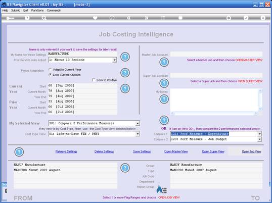
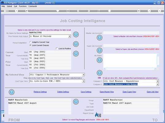
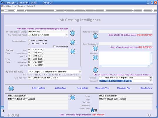
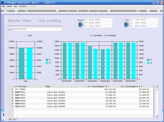
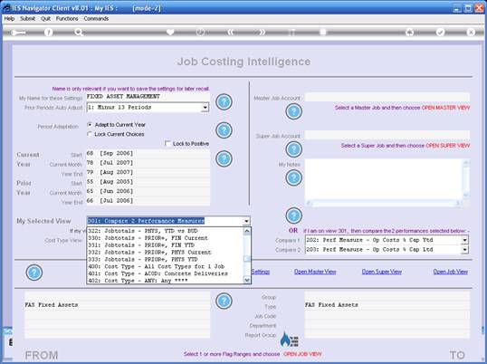
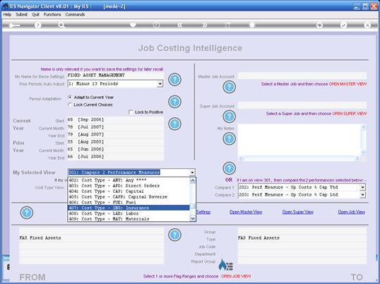
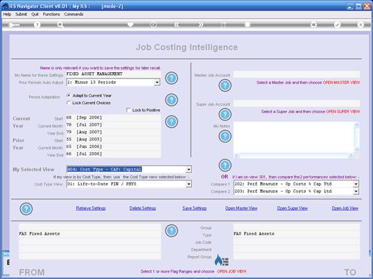
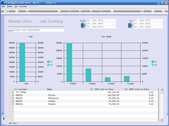
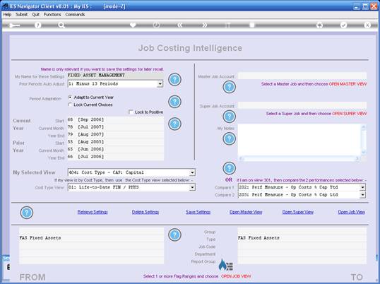
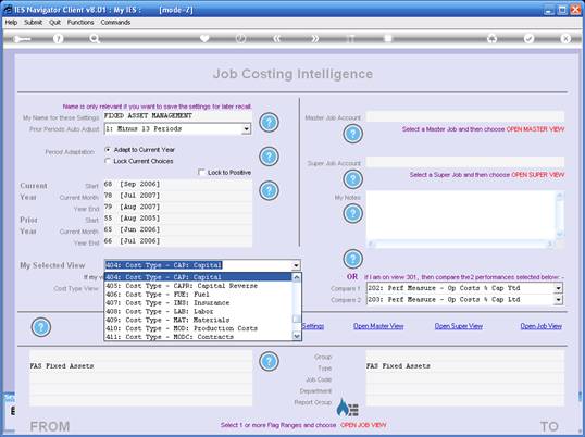
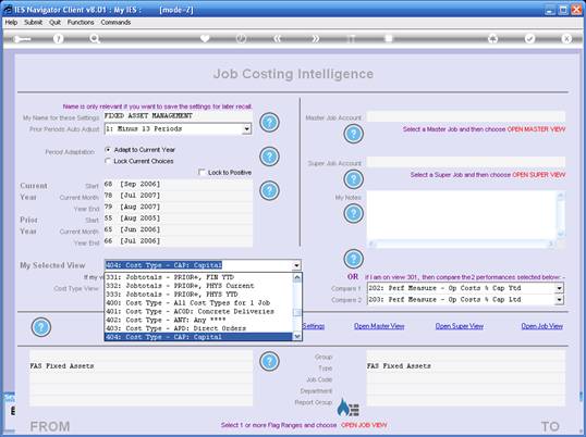
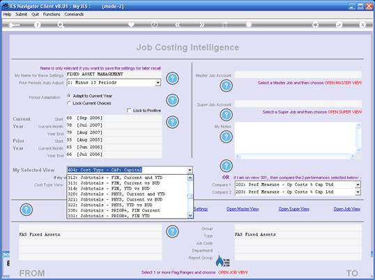
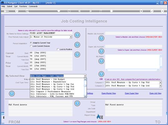
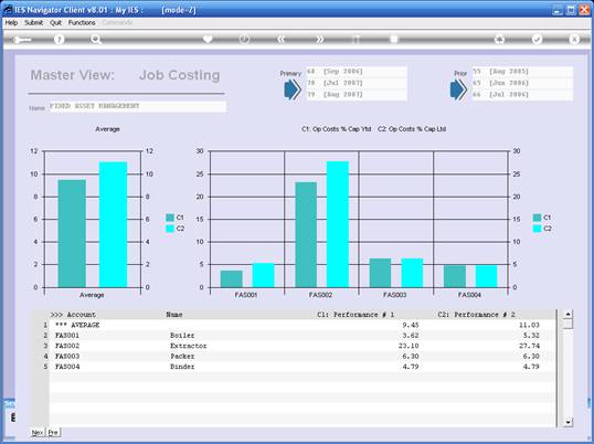
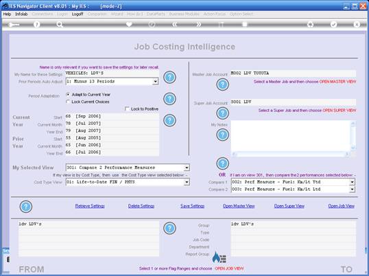
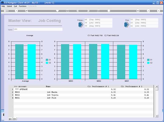
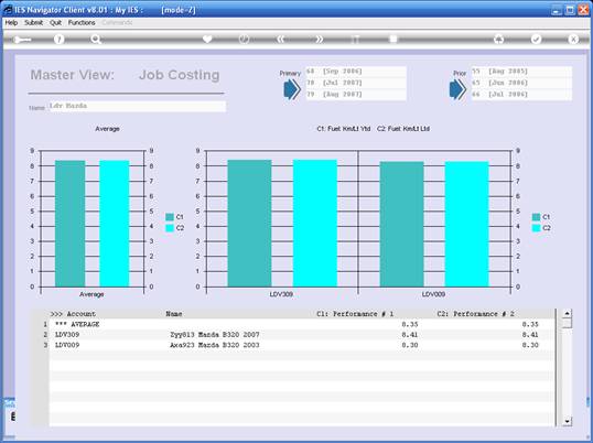
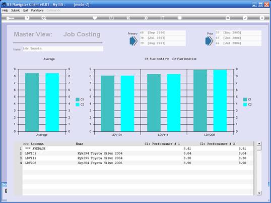
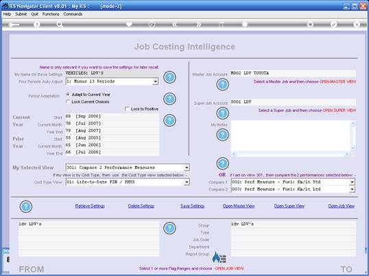
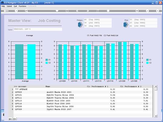
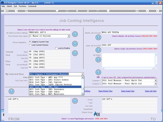
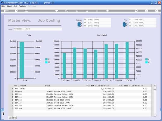
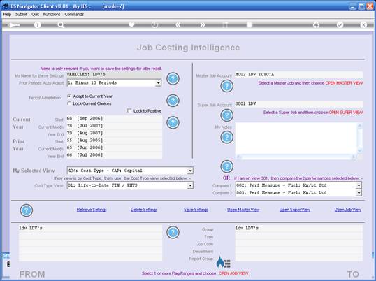
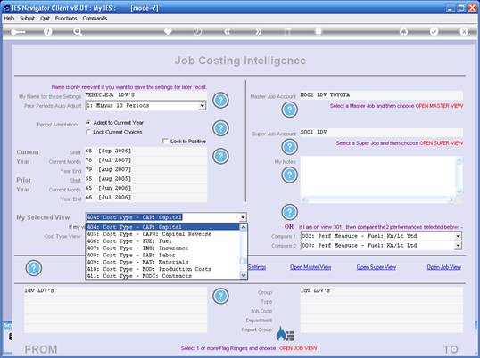
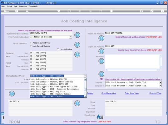
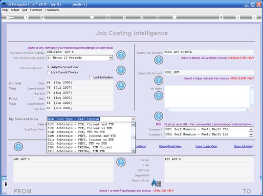
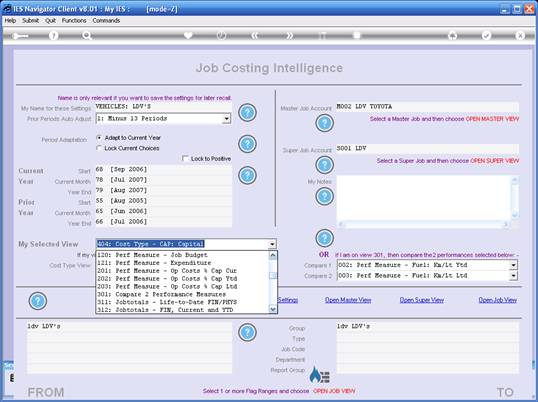
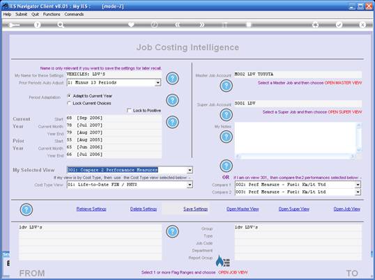
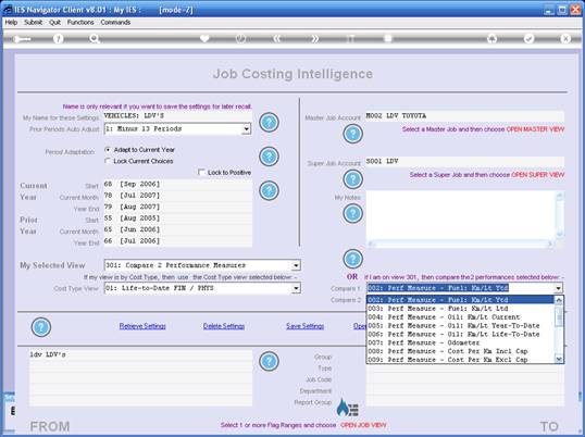
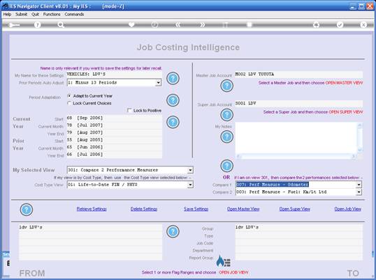
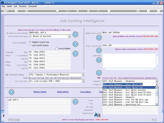
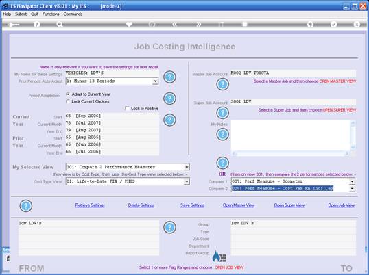
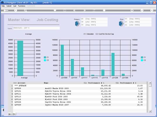
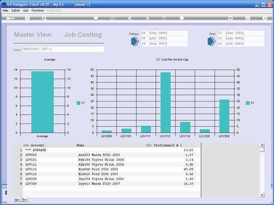
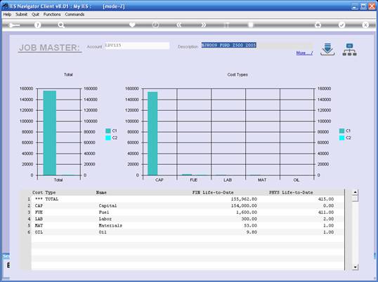
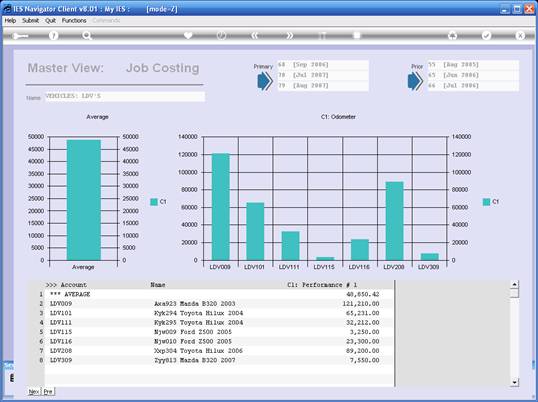
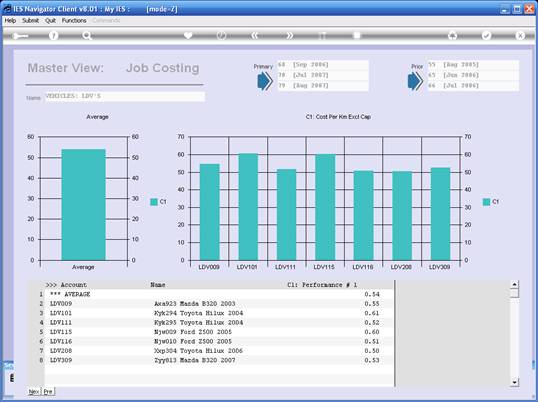
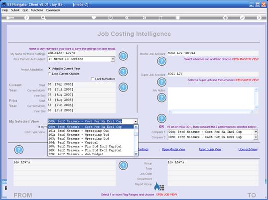
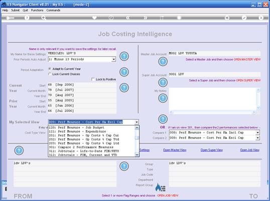
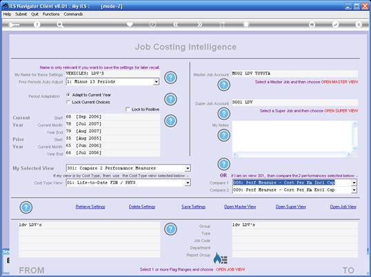
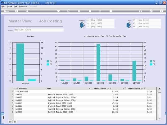
Slide notes: For Assets such as these, there are Lifetime Operational Expenditure that are in addition to the Capital Expenditure for the acquisition of the Assets. These Assets may break down, may need servicing, may use fuel, may need refurbishing, etc. It is the Operational Expenditure that we measure in the Job Costing system, and the Operational Expenditure as a factor of the original Capital Amount is an important measurement that can impact on any decision whether or not to replace an Asset.

Slide 56

Slide notes: This is our View of the Capital invested in these Asset Items.

Slide 57

Slide notes:

Slide 58

Slide notes:

Slide 59

Slide notes:

Slide 60

Slide notes:

Slide 61

Slide notes:

Slide 62

Slide notes:

Slide 63

Slide notes:

Slide 64

Slide notes:

Slide 65

Slide notes:

Slide 66

Slide notes: Here we have Operation Cost measured as a percentage of Capital Cost on a Year to Date and on a Life to Date basis. The 2nd Asset in the list stands out as being a quite high %, and we may want to drill into that Job to find out why.

Slide 67

Slide notes: Since Jobs may span multiple Financial Years and have Life to Date Views in addition to Year to Date Views, it means we can also measure Capital Project Budgets by Year as well as against the Lifetime Value.

Slide 68

Slide notes:

Slide 69

Slide notes:

Slide 70

Slide notes:

Slide 71

Slide notes: Our next example will be Fleet Management BI, so we will switch View Sets again.

Slide 72

Slide notes: For our View Set homing in on Light Delivery Vehicles in our Fleet, we lock onto the Job Group called LDV's, and we will also use examples of a Super Job and a Master Job, starting with the Super Job.

Slide 73

Slide notes:

Slide 74

Slide notes:

Slide 75

Slide notes:

Slide 76

Slide notes: A Super Job is always made up of 1 or more Master Jobs, and a Master Job is a pre-selection of Jobs.

Slide 77

Slide notes:

Slide 78

Slide notes:

Slide 79

Slide notes: By opening a Super Job View of our Light Delivery Vehicles, we are able to see average Fuel Performance for the various makes of LDV in our Fleet. Please note that the figures are fictitious, and for tutorial purposes only.

Slide 80

Slide notes: We can drill into any make of LDV here, to see the comparative figures for each LDV of that type.

Slide 81

Slide notes:

Slide 82

Slide notes:

Slide 83

Slide notes:

Slide 84

Slide notes:

Slide 85

Slide notes:

Slide 86

Slide notes:

Slide 87

Slide notes:

Slide 88

Slide notes: So we can see the averages for each Make of LDV at the Super Job level, and we can see the detail for each Make within the drillable Master Job View, but how can we see all the detail of all Makes of LDV together? No problem, we can just open the Job View.

Slide 89

Slide notes:

Slide 90

Slide notes:

Slide 91

Slide notes: And now we can see the results for all the Jobs in the LDV Group at the same time.

Slide 92

Slide notes: We can also see from the Vehicle Descriptions that they were acquired in different Years, therefore in all likelihood at quite different Prices. So we will quickly look at a View of the Capital invested in these Vehicles.

Slide 93

Slide notes:

Slide 94

Slide notes:

Slide 95

Slide notes:

Slide 96

Slide notes:

Slide 97

Slide notes:

Slide 98

Slide notes:

Slide 99

Slide notes: These then are the prices we paid to buy these Vehicles, and this will have an impact when we measure Operating Cost per Kilometer by including Capital Cost.

Slide 100

Slide notes:

Slide 101

Slide notes:

Slide 102

Slide notes:

Slide 103

Slide notes:

Slide 104

Slide notes:

Slide 105

Slide notes:

Slide 106

Slide notes:

Slide 107

Slide notes:

Slide 108

Slide notes:

Slide 109

Slide notes:

Slide 110

Slide notes:

Slide 111

Slide notes:

Slide 112

Slide notes: Now we find that the Capital Costs in this view dwarfs the Operating Cost per Kilometer. So let us have a look at the Cost per Kilometer on it's own.

Slide 113

Slide notes:

Slide 114

Slide notes:

Slide 115

Slide notes:

Slide 116

Slide notes:

Slide 117

Slide notes:

Slide 118

Slide notes:

Slide 119

Slide notes:

Slide 120

Slide notes:

Slide 121

Slide notes: And this is quite interesting. Immediately we want to ask how it is possible that the Vehicle on line 5 can be so high while the Vehicle on line 2 is so low! In fact, there is a very good explanation: it is because these figures are based on costs that INCLUDE the Capital, i.e. the new Price of the Vehicle. So any Vehicle with Low Mileage will have an inflated Cost Measurement when compared to a Vehicle with a Higher Mileage.

Slide 122

Slide notes:

Slide 123

Slide notes:

Slide 124

Slide notes: By drilling into the Vehicle Job, we get a Cost Type View. We can clearly see the Capital Cost, and the low Fuel amount, which implies low mileage, even though we cannot specifically see the mileage here. If need be, we can drill deeper into the Job Cost Types and Transactions.

Slide 125

Slide notes:

Slide 126

Slide notes:

Slide 127

Slide notes:

Slide 128

Slide notes:

Slide 129

Slide notes:

Slide 130

Slide notes:

Slide 131

Slide notes:

Slide 132

Slide notes:

Slide 133

Slide notes: On the Odometer View, we can now clearly see the low mileage at line 5. The Cost per Km measurement will be more realistic when we EXCLUDE the Capital Cost. Let's do that.

Slide 134

Slide notes:

Slide 135

Slide notes:

Slide 136

Slide notes:

Slide 137

Slide notes:

Slide 138

Slide notes: Indeed the picture looks more realistic now. For interest sake, we will now put the 2 measurements together in 1 View.

Slide 139

Slide notes:

Slide 140

Slide notes:

Slide 141

Slide notes:

Slide 142

Slide notes:

Slide 143

Slide notes:

Slide 144

Slide notes:

Slide 145

Slide notes:

Slide 146

Slide notes: And when we look at it like this, both with Capital Cost INcluded and EXcluded, we can see that the Vehicle on line 5 that raised the alarm initially, is in fact in the same band as the others when looked at without Capital Cost in the measurement.

Slide 147

Slide notes:

Slide 148

Slide notes: From these few examples, we hope to convey the message that the Job Costing BI can easily measure and reveal what we wish to know about Costing in our Business. Just imagine the question, and the answer can be revealed.